Kernel density estimation

 In statistics, kernel density estimation (KDE) is a non-parametric way to estimate the probability density function of a random variable. Kernel density estimation is a fundamental data smoothing problem where inferences about the population are made, based on a finite data sample. In some fields such as signal processing and econometrics it is also termed the Parzen–Rosenblatt window method, after Emanuel Parzen and Murray Rosenblatt, who are usually credited with independently creating it in its current form.^[1][2] One of the famous applications of kernel density estimation is in estimating the class-conditional marginal densities of data when using a naive Bayes classifier,^[3][4] which can improve its prediction accuracy.^[3]

Kernel density estimation of 100 normally distributed random numbers using different smoothing bandwidths.

DefinitionEdit

Let (x₁, x₂, …, x_n) be independent and identically distributed samples drawn from some univariate distribution with an unknown density ƒ at any given point x. We are interested in estimating the shape of this function ƒ. Its kernel density estimator is

${\displaystyle {\widehat {f}}_{h}(x)={\frac {1}{n}}\sum _{i=1}^{n}K_{h}(x-x_{i})={\frac {1}{nh}}\sum _{i=1}^{n}K{\Big (}{\frac {x-x_{i}}{h}}{\Big )},}$

where K is the kernel — a non-negative function — and h > 0 is a smoothing parameter called the bandwidth. A kernel with subscript h is called the scaled kernel and defined as K_h(x) = 1/h K(x/h). Intuitively one wants to choose h as small as the data will allow; however, there is always a trade-off between the bias of the estimator and its variance. The choice of bandwidth is discussed in more detail below.

A range of kernel functions are commonly used: uniform, triangular, biweight, triweight, Epanechnikov, normal, and others. The Epanechnikov kernel is optimal in a mean square error sense,^[5] though the loss of efficiency is small for the kernels listed previously.^[6] Due to its convenient mathematical properties, the normal kernel is often used, which means K(x) = ϕ(x), where ϕ is the standard normal density function.

The construction of a kernel density estimate finds interpretations in fields outside of density estimation.^[7] For example, in thermodynamics, this is equivalent to the amount of heat generated when heat kernels (the fundamental solution to the heat equation) are placed at each data point locations x_i. Similar methods are used to construct discrete Laplace operators on point clouds for manifold learning (e.g. diffusion map).

ExampleEdit

Kernel density estimates are closely related to histograms, but can be endowed with properties such as smoothness or continuity by using a suitable kernel. An example using 6 data points illustrates this difference between histogram and kernel density estimators:

Sample	1	2	3	4	5	6
Value	-2.1	-1.3	-0.4	1.9	5.1	6.2

For the histogram, first the horizontal axis is divided into sub-intervals or bins which cover the range of the data: In this case, six bins each of width 2. Whenever a data point falls inside this interval, a box of height 1/12 is placed there. If more than one data point falls inside the same bin, the boxes are stacked on top of each other.

For the kernel density estimate, a normal kernel with standard deviation 2.25 (indicated by the red dashed lines) is placed on each of the data points x_i. The kernels are summed to make the kernel density estimate (solid blue curve). The smoothness of the kernel density estimate (compared to the discreteness of the histogram) illustrates how kernel density estimates converge faster to the true underlying density for continuous random variables.^[8]

Comparison of the histogram (left) and kernel density estimate (right) constructed using the same data. The six individual kernels are the red dashed curves, the kernel density estimate the blue curves. The data points are the rug plot on the horizontal axis.

Bandwidth selectionEdit

Kernel density estimate (KDE) with different bandwidths of a random sample of 100 points from a standard normal distribution. Grey: true density (standard normal). Red: KDE with h=0.05. Black: KDE with h=0.337. Green: KDE with h=2.

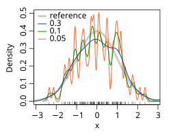
The bandwidth of the kernel is a free parameter which exhibits a strong influence on the resulting estimate. To illustrate its effect, we take a simulated random sample from the standard normal distribution (plotted at the blue spikes in the rug plot on the horizontal axis). The grey curve is the true density (a normal density with mean 0 and variance 1). In comparison, the red curve is undersmoothed since it contains too many spurious data artifacts arising from using a bandwidth h = 0.05, which is too small. The green curve is oversmoothed since using the bandwidth h = 2 obscures much of the underlying structure. The black curve with a bandwidth of h = 0.337 is considered to be optimally smoothed since its density estimate is close to the true density. An extreme situation is encountered in the limit ${\displaystyle h\to 0}$ (no smoothing), where the estimate is a sum of n delta functions centered at the coordinates of analyzed samples. In the other extreme limit ${\displaystyle h\to \infty }$ the estimate retains the shape of the used kernel, centered on the mean of the samples (completely smooth).

The most common optimality criterion used to select this parameter is the expected L₂ risk function, also termed the mean integrated squared error:

${\displaystyle \operatorname {MISE} (h)=\operatorname {E} \!\left[\,\int ({\hat {f}}_{h}(x)-f(x))^{2}\,dx\right].}$

Under weak assumptions on ƒ and K, (ƒ is the, generally unknown, real density function),^[1][2] MISE (h) = AMISE(h) + o(1/(nh) + h⁴) where o is the little o notation. The AMISE is the Asymptotic MISE which consists of the two leading terms

${\displaystyle \operatorname {AMISE} (h)={\frac {R(K)}{nh}}+{\frac {1}{4}}m_{2}(K)^{2}h^{4}R(f'')}$

where ${\displaystyle R(g)=\int g(x)^{2}\,dx}$ for a function g, ${\displaystyle m_{2}(K)=\int x^{2}K(x)\,dx}$ and ƒ'' is the second derivative of ƒ. The minimum of this AMISE is the solution to this differential equation

${\displaystyle {\frac {\partial }{\partial h}}\operatorname {AMISE} (h)=-{\frac {R(K)}{nh^{2}}}+m_{2}(K)^{2}h^{3}R(f'')=0}$

or

${\displaystyle h_{\operatorname {AMISE} }={\frac {R(K)^{1/5}}{m_{2}(K)^{2/5}R(f'')^{1/5}n^{1/5}}}.}$

Neither the AMISE nor the h_AMISE formulas are able to be used directly since they involve the unknown density function ƒ or its second derivative ƒ'', so a variety of automatic, data-based methods have been developed for selecting the bandwidth. Many review studies have been carried out to compare their efficacies,^{[9][10][11][12][13][14][15]} with the general consensus that the plug-in selectors^[7][16][17] and cross validation selectors^[18][19][20] are the most useful over a wide range of data sets.

Substituting any bandwidth h which has the same asymptotic order n^−1/5 as h_AMISE into the AMISE gives that AMISE(h) = O(n^−4/5), where O is the big o notation. It can be shown that, under weak assumptions, there cannot exist a non-parametric estimator that converges at a faster rate than the kernel estimator.^[21] Note that the n^−4/5 rate is slower than the typical n⁻¹ convergence rate of parametric methods.

If the bandwidth is not held fixed, but is varied depending upon the location of either the estimate (balloon estimator) or the samples (pointwise estimator), this produces a particularly powerful method termed adaptive or variable bandwidth kernel density estimation.

Bandwidth selection for kernel density estimation of heavy-tailed distributions is relatively difficult.^[22]

A rule-of-thumb bandwidth estimatorEdit

If Gaussian basis functions are used to approximate univariate data, and the underlying density being estimated is Gaussian, the optimal choice for h (that is, the bandwidth that minimises the mean integrated squared error) is:^[23]

${\displaystyle h=\left({\frac {4{\hat {\sigma }}^{5}}{3n}}\right)^{\frac {1}{5}}\approx 1.06\,{\hat {\sigma }}\,n^{-1/5},}$

In order to make the h value more robust to make the fitness well for both long-tailed and skew distribution and bimodal mixture distribution, it is better to substitute the value of ${\displaystyle {\hat {\sigma }}}$ with another parameter A, which is given by:

A = min(standard deviation, interquartile range/1.34).

Another modification that will improve the model is to reduce the factor from 1.06 to 0.9. Then the final formula would be:

${\displaystyle h=0.9\,\min \left({\hat {\sigma }},{\frac {IQR}{1.34}}\right)\,n^{\frac {-1}{5}}}$

where ${\displaystyle {\hat {\sigma }}}$ is the standard deviation of the samples, n is the sample size. IQR is the interquartile range.

This approximation is termed the normal distribution approximation, Gaussian approximation, or Silverman's rule of thumb.^[23] While this rule of thumb is easy to compute, it should be used with caution as it can yield widely inaccurate estimates when the density is not close to being normal. For example, when estimating the bimodal Gaussian mixture model

Comparison between rule of thumb and solve-the-equation bandwidth.

${\displaystyle \textstyle {\frac {1}{2{\sqrt {2\pi }}}}e^{-{\frac {1}{2}}(x-10)^{2}}+{\frac {1}{2{\sqrt {2\pi }}}}e^{-{\frac {1}{2}}(x+10)^{2}}}$

from a sample of 200 points. The figure on the right shows the true density and two kernel density estimates—one using the rule-of-thumb bandwidth, and the other using a solve-the-equation bandwidth.^[7][17] The estimate based on the rule-of-thumb bandwidth is significantly oversmoothed.

Relation to the characteristic function density estimatorEdit

Given the sample (x₁, x₂, …, x_n), it is natural to estimate the characteristic function φ(t) = E[e^itX] as

${\displaystyle {\widehat {\varphi }}(t)={\frac {1}{n}}\sum _{j=1}^{n}e^{itx_{j}}}$

Knowing the characteristic function, it is possible to find the corresponding probability density function through the Fourier transform formula. One difficulty with applying this inversion formula is that it leads to a diverging integral, since the estimate ${\displaystyle \scriptstyle {\widehat {\varphi }}(t)}$ is unreliable for large t’s. To circumvent this problem, the estimator ${\displaystyle \scriptstyle {\widehat {\varphi }}(t)}$ is multiplied by a damping function ψ_h(t) = ψ(ht), which is equal to 1 at the origin and then falls to 0 at infinity. The “bandwidth parameter” h controls how fast we try to dampen the function ${\displaystyle \scriptstyle {\widehat {\varphi }}(t)}$. In particular when h is small, then ψ_h(t) will be approximately one for a large range of t’s, which means that ${\displaystyle \scriptstyle {\widehat {\varphi }}(t)}$ remains practically unaltered in the most important region of t’s.

The most common choice for function ψ is either the uniform function ψ(t) = 1{−1 ≤ t ≤ 1}, which effectively means truncating the interval of integration in the inversion formula to [−1/h, 1/h], or the Gaussian function ψ(t) = e^−πt2. Once the function ψ has been chosen, the inversion formula may be applied, and the density estimator will be

${\displaystyle {\begin{aligned}{\widehat {f}}(x)&={\frac {1}{2\pi }}\int _{-\infty }^{+\infty }{\widehat {\varphi }}(t)\psi _{h}(t)e^{-itx}\,dt={\frac {1}{2\pi }}\int _{-\infty }^{+\infty }{\frac {1}{n}}\sum _{j=1}^{n}e^{it(x_{j}-x)}\psi (ht)\,dt\\[5pt]&={\frac {1}{nh}}\sum _{j=1}^{n}{\frac {1}{2\pi }}\int _{-\infty }^{+\infty }e^{-i(ht){\frac {x-x_{j}}{h}}}\psi (ht)\,d(ht)={\frac {1}{nh}}\sum _{j=1}^{n}K{\Big (}{\frac {x-x_{j}}{h}}{\Big )},\end{aligned}}}$

where K is the Fourier transform of the damping function ψ. Thus the kernel density estimator coincides with the characteristic function density estimator.

Geometric and topological featuresEdit

We can extend the definition of the (global) mode to a local sense and define the local modes:

${\displaystyle M=\{x:g(x)=0,\lambda _{1}(x)<0\}}$

Namely, ${\displaystyle M}$ is the collection of points for which the density function is locally maximized. A natural estimator of ${\displaystyle M}$ is a plug-in from KDE,^[24][25] where ${\displaystyle g(x)}$ and ${\displaystyle \lambda _{1}(x)}$ are KDE version of ${\displaystyle g(x)}$ and ${\displaystyle \lambda _{1}(x)}$. Under mild assumptions, ${\displaystyle M_{c}}$ is a consistent estimator of ${\displaystyle M}$. Note that one can use the mean shift algorithm^[26][27][28] to compute the estimator ${\displaystyle M_{c}}$ numerically.

This article uses material from the Wikipedia article  Metasyntactic variable, which is released under the  Creative Commons Attribution-ShareAlike 3.0 Unported License.