Unsupervised learning

 Unsupervised learning (UL) is a type of algorithm that learns patterns from untagged data. The hope is that through mimicry, the machine is forced to build a compact internal representation of its world. In contrast to Supervised Learning (SL) where data is tagged by a human, eg. as "car" or "fish" etc, UL exhibits self-organization that captures patterns as neuronal predelections or probability densities.^[1] The other levels in the supervision spectrum are Reinforcement Learning where the machine is given only a numerical performance score as its guidance, and Semi-supervised learning where a smaller portion of the data is tagged. Two broad methods in UL are Neural Networks and Probabilistic Methods.

Probabilistic methodsEdit

Two of the main methods used in unsupervised learning are principal component and cluster analysis. Cluster analysis is used in unsupervised learning to group, or segment, datasets with shared attributes in order to extrapolate algorithmic relationships.^[2] Cluster analysis is a branch of machine learning that groups the data that has not been labelled, classified or categorized. Instead of responding to feedback, cluster analysis identifies commonalities in the data and reacts based on the presence or absence of such commonalities in each new piece of data. This approach helps detect anomalous data points that do not fit into either group.

The only requirement to be called an unsupervised learning strategy is to learn a new feature space that captures the characteristics of the original space by maximizing some objective function or minimising some loss function. Therefore, generating a covariance matrix is not unsupervised learning, but taking the eigenvectors of the covariance matrix is because the linear algebra eigendecomposition operation maximizes the variance; this is known as principal component analysis.^[3] Similarly, taking the log-transform of a dataset is not unsupervised learning, but passing input data through multiple sigmoid functions while minimising some distance function between the generated and resulting data is, and is known as an Autoencoder.

A central application of unsupervised learning is in the field of density estimation in statistics,^[4] though unsupervised learning encompasses many other domains involving summarizing and explaining data features. It could be contrasted with supervised learning by saying that whereas supervised learning intends to infer a conditional probability distribution ${\textstyle p_{X}(x\,|\,y)}$ conditioned on the label ${\textstyle y}$ of input data; unsupervised learning intends to infer an a priori probability distribution ${\textstyle p_{X}(x)}$.

ApproachesEdit

Some of the most common algorithms used in unsupervised learning include: (1) Clustering, (2) Anomaly detection, (3) Neural Networks, and (4) Approaches for learning latent variable models. Each approach uses several methods as follows:

• Clustering methods include: hierarchical clustering,^[5] k-means,^[6] mixture models, DBSCAN, and OPTICS algorithm
• Anomaly detection methods include: Local Outlier Factor, and Isolation Forest
• Approaches for learning latent variable models such as Expectation–maximization algorithm (EM), Method of moments, and Blind signal separation techniques ( Principal component analysis, Independent component analysis, Non-negative matrix factorization, Singular value decomposition )

Method of momentsEdit

One of the statistical approaches for unsupervised learning is the method of moments. In the method of moments, the unknown parameters (of interest) in the model are related to the moments of one or more random variables, and thus, these unknown parameters can be estimated given the moments. The moments are usually estimated from samples empirically. The basic moments are first and second order moments. For a random vector, the first order moment is the mean vector, and the second order moment is the covariance matrix (when the mean is zero). Higher order moments are usually represented using tensors which are the generalization of matrices to higher orders as multi-dimensional arrays.

In particular, the method of moments is shown to be effective in learning the parameters of latent variable models.^[7] Latent variable models are statistical models where in addition to the observed variables, a set of latent variables also exists which is not observed. A highly practical example of latent variable models in machine learning is the topic modeling which is a statistical model for generating the words (observed variables) in the document based on the topic (latent variable) of the document. In the topic modeling, the words in the document are generated according to different statistical parameters when the topic of the document is changed. It is shown that method of moments (tensor decomposition techniques) consistently recover the parameters of a large class of latent variable models under some assumptions.^[7]

The Expectation–maximization algorithm (EM) is also one of the most practical methods for learning latent variable models. However, it can get stuck in local optima, and it is not guaranteed that the algorithm will converge to the true unknown parameters of the model. In contrast, for the method of moments, the global convergence is guaranteed under some conditions.^[7]

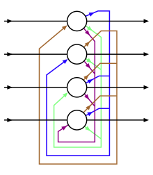
Neural networksEdit

BasicsEdit

First, some vocabulary:

activation	= state value of the neuron. For binary neurons, this is usually 0 / 1, or +1 / -1.
CAM	= content addressable memory. Recalling a memory by a partial pattern instead of a memory address.
convergence	= the stabilization of an activation pattern on a network. In SL, convergence means stabilization of weights & biases rather than activations.
discriminative	= relating to recognition tasks. Also called analysis (in Pattern Theory), or inference.
energy	= a macroscopic quantity describing the activation pattern in a network. (see below)
generalization	= behaving accurately on unseen inputs
generative	= Machine imagined and recall task. sometimes called synthesis (in Pattern Theory), mimicry, or deep fakes.
inference	= the "run" phase (as opposed to training). During inference the network performs the task it is trained to do—either recognizing a pattern (SL) or creating one (UL). Usually inference descends the gradient of an energy function. In contrast to SL, gradient descent occurs during training, NOT inference.
machine vision	= machine learning on images.
NLP	= Natural Language Processing. Machine learning of human languages.
pattern	= network activations that has an internal order in some sense, or that can be described more compactly by features in the activations. For example, the pixel pattern of a zero, whether it's given as data or imagined by the network, has a feature that is describable as a single loop. The features are encoded in the hidden neurons.
training	= the learning phase. Here, the network adjusts its weights & biases to learn from the inputs.

Tasks

Tendency for a task to employ Supervised vs. Unsupervised methods

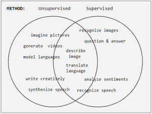
UL methods usually prepare a network for generative tasks rather than recognition, but grouping tasks as supervised or not can be hazy. For example, handwriting recognition started off in the 1980s as SL. Then in 2007, UL is used to prime the network for SL afterwards. Currently, SL has regained its position as the better method.

Training
During the learning phase, an unsupervised network tries to mimic the data it's given and uses the error in its mimicked output to correct itself (eg. its weights & biases). This resembles the mimicry behavior of children as they learn a language. Sometimes the error is expressed as a low probability that the erroneous output occurs, or it might be express as an unstable high energy state in the network.

Energy
An energy function is a macroscopic measure of a network's state. This analogy with physics is inspired by Ludwig Boltzmann's analysis of a gas' macroscopic energy from the microscopic probabilities of particle motion p ${\displaystyle \propto }$ e^E/kT, where k is the Boltzmann constant and T is temperature. In neural networks the relation is p = e^-E / Z, where p & E vary over every possible input pattern. Hence, early neural networks bear the name Boltzmann Machine. Paul Smolensky calls -E the Harmony. A network seeks low energy which is high Harmony.

Networks

Hopfield	Boltzmann	RBM	Helmholtz	Autoencoder	VAE
		restricted Boltzmann machine		autoencoder	variational autoencoder

Boltzmann and Helmholtz came before neural networks formulations, but these networks borrowed from their analyses, so these networks bear their names. Hopfield, however, directly contributed to UL.

IntermediateEdit

Here, distributions p(x) and q(x) will be abbreviated as p and q.

History

1969	Perceptrons by Minsky & Papert shows a perceptron without hidden layers fails on XOR
1970s	(approximate dates) AI winter I
1974	Ising magnetic model proposed by WA Little for cognition
1980	Fukushima introduces the neocognitron, which is later called a convolution neural network. It is mostly used in SL, but deserves a mention here.
1982	Ising variant Hopfield net described as CAMs and classifiers by John Hopfield.
1983	Ising variant Boltzmann machine with probabilistic neurons described by Hinton & Sejnowski following Sherington & Kirkpatrick's 1975 work.
1986	Paul Smolensky publishes Harmony Theory, which is an RBM with practically the same Boltzmann energy function. Smolensky did not give an practical training scheme. Hinton did in mid-2000s
1995	Schmidthuber introduces the LSTM neuron for languages.
1995	Dayan & Hinton introduces Helmholtz machine
1995-2005	(approximate dates) AI winter II
2013	Kingma, Rezende, & co. introduced Variational Autoencoders as Bayesian graphical probability network, with neural nets as components.

Some more vocabulary:

Probability
cdf	= cumulative distribution function. the integral of the pdf. The probability of getting near 3 is the area under the curve between 2.9 and 3.1.
contrastive divergence	= a learning method where one lowers the energy on training patterns and raises the energy on unwanted patterns outside of the training set. This is very different from the KL-divergence, but shares a similar wording.
expected value	= E(x) = ${\displaystyle \sum _{x}}$ x * p(x). This is the mean value, or average value. For continuous input x, replace the summation with an integral.
latent variable	= an unobserved quantity that helps to explain observed data. for instance, a flu infection (unobserved) can explain why the a person sneezes (observed). In probabilistic neural networks, hidden neurons act as latent variables, though their latent interpretation is not explicitly known.
pdf	= probability density function. The probability that a random variable takes on a certain value. For continuous pdf, p(3) = 1/2 can still mean there is near zero chance of achieving this exact value of 3. We rationalize this with the cdf.
stochastic	= behaves according to a well described probability density formula.
Thermodynamics
Boltzmann distribution	= Gibbs distribution. p ${\displaystyle \propto }$ eE/kT
entropy	= expected information = ${\displaystyle \sum _{x}}$ p * log p
Gibbs free energy	= thermodynamic potential. It's the maximum reversible work that may be performed by a heat system at constant temperature and pressure. free energy G = heat - temperature * entropy
information	= the information amount of a message x = -log p(x)
KLD	= relative entropy. For probabilistic networks, this is the analogue of the error between input & mimicked output. The Kullback-Liebler divergence (KLD) measures the entropy deviation of 1 distribution from another distribution. KLD(p,q) = ${\displaystyle \sum _{x}}$ p * log( p / q ). Typically, p reflects the input data, q reflects the network's interpretation of it, and KLD reflects the difference between the two.

Comparison of Networks

	Hopfield	Boltzmann	RBM	Helmholtz	Autoencoder	VAE
usage & notables	CAM, traveling salesman problem	CAM. The freedom of connections makes this network difficult to analyze.	pattern recognition (MNIST, speech recognition)	imagination, mimicry	language: creative writing, translation. Vision: enhancing blurry images	generate realistic data
neuron	deterministic binary state. Activation = { 0 (or -1) if x is negative, 1 otherwise }	stochastic binary Hopfield neuron	stochastic binary. Extended to real-valued in mid 2000s	binary, sigmoid	language: LSTM. vision: local receptive fields. usually real valued relu activation.
connections	1-layer with symmetric weights. No self-connections.	2-layers. 1-hidden & 1-visible. symmetric weights.	2-layers. symmetric weights. no lateral connections within a layer.	3-layers: asymmetric weights. 2 networks combined into 1.	3-layers. The input is considered a layer even though it has no inbound weights. recurrent layers for NLP. feedforward convolutions for vision. input & output have the same neuron counts.	3-layers: input, encoder, distribution sampler decoder. the sampler is not considered a layer (e)
inference & energy	energy is given by Gibbs probability measure :${\displaystyle E=-{\frac {1}{2}}\sum _{i,j}{w_{ij}{s_{i}}{s_{j}}}+\sum _{i}{\theta _{i}}{s_{i}}}$	← same	← same	minimize KL divergence	inference is only feed-forward. previous UL networks ran forwards AND backwards	minimize error = reconstruction error - KLD
training	Δwij = si*sj, for +1/-1 neuron	Δwij = e*(pij - p'ij). This is derived from minimizing KLD. e = learning rate, p' = predicted and p = actual distribution.	contrastive divergence w/ Gibbs Sampling	wake-sleep 2 phase training	back propagate the reconstruction error	reparameterize hidden state for backprop
strength	resembles physical systems so it inherits their equations	<--- same. hidden neurons act as internal representatation of the external world	faster more practical training scheme than Boltzmann machines	mildly anatomical. analyzable w/ information theory & statistical mechanics
weakness	hopfield	hard to train due to lateral connections	RBM	Helmholtz

Specific Networks
Here, we highlight some characteristics of each networks. Ferromagnetism inspired Hopfield networks, Boltzmann machines, and RBMs. A neuron correspond to an iron domain with binary magnetic moments Up and Down, and neural connections correspond to the domain's influence on each other. Symmetric connections enables a global energy formulation. During inference the network updates each state using the standard activation step function. Symmetric weights guarantees convergence to a stable activation pattern.
Hopfield networks are used as CAMs and are guaranteed to settle to a some pattern. Without symmetric weights, the network is very hard to analyze. With the right energy function, a network will converge.
Boltzmann machines are stochastic Hopfield nets. Their state value is sampled from this pdf as follows: suppose a binary neuron fires with the Bernoulli probability p(1) = 1/3 and rests with p(0) = 2/3. One samples from it by taking a UNIFORMLY distributed random number y, and plugging it into the inverted cumulative distribution function, which in this case is the step function thresholded at 2/3. The inverse function = { 0 if x <= 2/3, 1 if x > 2/3 }
Helmholtz machines are early inspirations for the Variational Auto Encoders. It's 2 networks combined into one—forward weights operates recognition and backward weights implements imagination. It is perhaps the first network to do both. Helmholtz did not work in machine learning but he inspired the view of "statistical inference engine whose function is to infer probable causes of sensory input" (3). the stochastic binary neuron outputs a probability that its state is 0 or 1. The data input is normally not considered a layer, but in the Helmholtz machine generation mode, the data layer receives input from the middle layer has separate weights for this purpose, so it is considered a layer. Hence this network has 3 layers.
Variational Autoencoder (VAE) are inspired by Helmholtz machines and combines probability network with neural networks. An Autoencoder is a 3-layer CAM network, where the middle layer is supposed to be some internal representation of input patterns. The weights are named phi & theta rather than W and V as in Helmholtz—a cosmetic difference. The encoder neural network is a probability distribution q_φ(z|x) and the decoder network is p_θ(x|z). These 2 networks here can be fully connected, or use another NN scheme.

Hebbian Learning, ART, SOM
The classical example of unsupervised learning in the study of neural networks is Donald Hebb's principle, that is, neurons that fire together wire together.^[8] In Hebbian learning, the connection is reinforced irrespective of an error, but is exclusively a function of the coincidence between action potentials between the two neurons.^[9] A similar version that modifies synaptic weights takes into account the time between the action potentials (spike-timing-dependent plasticity or STDP). Hebbian Learning has been hypothesized to underlie a range of cognitive functions, such as pattern recognition and experiential learning.

Among neural network models, the self-organizing map (SOM) and adaptive resonance theory (ART) are commonly used in unsupervised learning algorithms. The SOM is a topographic organization in which nearby locations in the map represent inputs with similar properties. The ART model allows the number of clusters to vary with problem size and lets the user control the degree of similarity between members of the same clusters by means of a user-defined constant called the vigilance parameter. ART networks are used for many pattern recognition tasks, such as automatic target recognition and seismic signal processing.^[10]

This article uses material from the Wikipedia article  Metasyntactic variable, which is released under the  Creative Commons Attribution-ShareAlike 3.0 Unported License.